Pontification about inflation of prices of goods and services is on a rampage. Almost all the noise is based on inadequate inflation theory. A more complete approach is presented at length in Taylor and Barbosa-Filho (2021) and summarized here.
In early 2021, individual price jumps spread across the economy. They have not yet fed into a “cumulative process” inflation as described more than a century ago by the Swedish economist Knut Wicksell.
To grasp Wickell’s analysis, we can employ a small modification of standard national income and product (NIPA) accounts. The value of total “supply” (price index times real quantity) is nominal gross domestic product (GDP) plus imports. The cost of supply is nominal gross domestic income (GDI or wages, profits, and indirect taxes) plus imports. Ignoring “errors and omissions,” the key balancing requirement in the NIPA is GDP equals GDI.
We can divide the value of supply by its real level, leaving the price index. The same maneuver for the cost of supply gives the sum of a profit mark-up; unit labor cost (nominal wage divided by the output/labor ratio or labor productivity); import cost (world price times the exchange rate times the import/supply ratio); and indirect tax divided by supply.
Numbers are presented below. The key implication of the accounting is that exponential growth of the price level has to be accompanied by exponential growth of components of cost, specifically unit labor and import cost. With price increases setting off cost increases which feed into higher prices, a Wicksellian cumulative process is underway. Such dynamics have not occurred in the USA since the stagflation period in the 1960s and 1970s. They may or may not show up again.
Implications of inflation
A few further observations are in order.
Inflation as noted is a dynamical process, meaning it has to be understood historically. Its exponential growth comes from positive feedback between prices and costs.
The dynamics often arise from social conflict. Higher profits and import costs cut into the wage share of GDI and unit labor cost. Rising import and wage costs can provoke destabilizing price dynamics driven by increasing nominal GDI. Conflict over wages vs profits and assets vs liabilities in balance sheets can drive price inflation. Income claims were at stake during the American stagflation period before 1980. High debt with price deflation drove William Jennings Bryan to make his famous Cross of Gold speech in 1896.
Stabilizing inflation, as with Paul Volcker’s shock treatment around 40 years ago (itself based on developing country stabilizations pioneered by the International Monetary Fund three decades before 1980), almost always relies on tight money and wage suppression which began around 1970 in the USA (Taylor with Ömer, 2020).
At present, loose money and potential upward wage movements could set off serious price inflation which in turn would pull up the interest rate. A low interest rate has over the past three decades supported high prices of assets (real estate and corporate shares). Wall Street has benefitted and would oppose interest rate increases in response to more inflation.
Cost-based analysis has not figured in American inflation discussion post-Volcker. Rather, economists pursued will-o’-the-wisp including inflation expectations and an incorrectly specified Phillips curve as discussed below.
The Biden administration could well face a policy trilemma involving (i) the only path toward a more egalitarian size distribution of income is through a rising labor share (money wage growth exceeds price plus productivity growth), (ii) which would provoke faster inflation with feedback to rising interest rates, and (iii) resulting asset price deflation facing likely political resistance from Wall Street and affluent households.
Structure of costs
We can begin with the macroeconomic structure of costs, as shown in Figure 1. There were quarterly jumps of the consumer price index (CPI) inflation rate toward twenty percent per year during and after both World Wars. They soon subsided. The diagram illustrates the process post-1947. Components of cost are imports; payments to labor including “supplements” for insurance, pensions, etc., paid by employers; indirect taxes; and gross capital income including corporate profits, payments to proprietors, etc.
Indexes are on a log scale, with cost per unit output at 100 in 1960. In the diagram, the labor share has consistently been pressed “from below” by rising imports and “from above” by increasing business taxes and gross profits. The wage share of GDI has been falling since around 1970. This trend contributed to the success of the Volcker stabilization package.
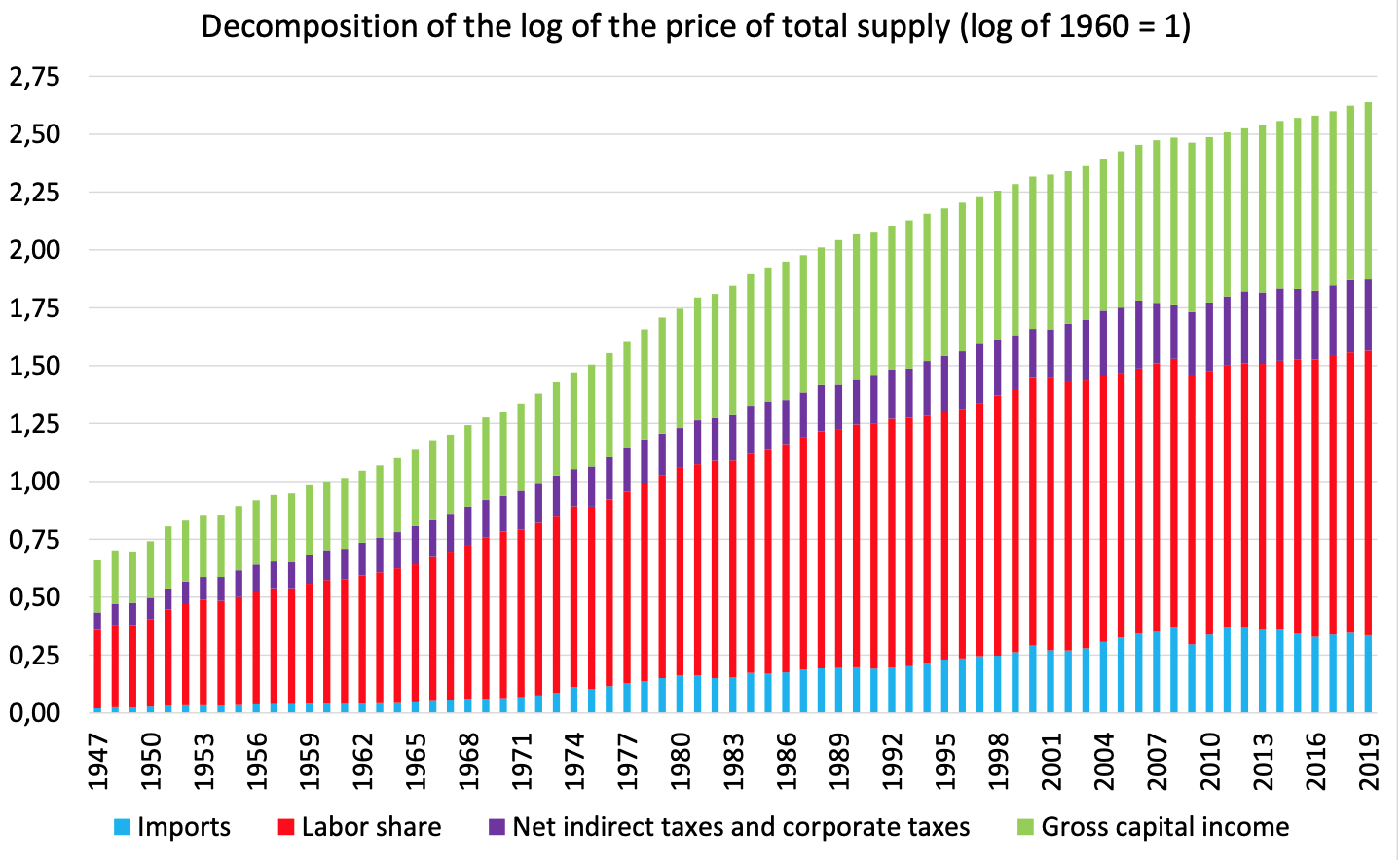
Figure 1: Log of the cost of total supply. Note how labor cost after 1970 is squeezed “from below” by rising imports and “from above” by profits.
Inflation post-Volcker
Volcker’s stabilization knocked the annual GDP growth rate below minus four percent in 1982. Figure 2 shows what happened to the price level and costs. The GDP deflator is used as the price index because it reflects costs of production better than the consumer price index. The relevant comparison is between money wage inflation and the sum of price inflation and the rate of productivity growth since the latter reduces costs. The diagram shows that after the 1970s wages lagged prices and productivity, leading to a decrease in the labor share. Over five decades, the share fell by about five percentage points (Taylor with Ömer, 2020). It does vary pro-cyclically (less strongly in recent years) as pointed out by Barbosa-Filho and Taylor (2006), among many others.
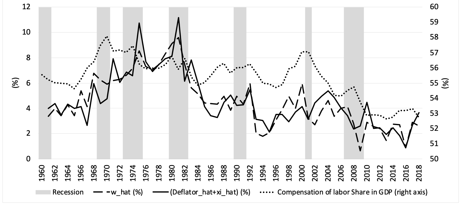
Figure 2: Money wage growth (w_hat) vs. GDP deflator growth plus productivity growth (deflator_hat+xi_hat) and the labor share including “supplements”
After the mid-1980s the general picture is one of stable, slowly declining inflation, in sharp contrast to the stagflation period between 1960 and 1980. Figure 1 shows that those two decades featured rising labor and import costs. Stopping inflation was inevitable, given the American political economy. Volcker was hired to do the job, He did it efficiently using tools off the IMF shelf.
Without major inflation concerns post-1985, academic economists like generals turned to fighting yesterday’s wars. The twist is that the Fed took them seriously, basing monetary policy on ideas about stagflation from Chicago and MIT. Active discussion focused on expectations and the Phillips curve. Both linked inflation to the level of economic activity, ignoring the structure of costs.
Inflation expectations
In his General Theory, Keynes (1936) used the word “expectation” to describe shared opinion about the state of the economy. Because it reflected a social consensus expectation could be stable for a period of time, but then change rapidly.[1] After WWII, economists transformed “expectations” to signify the mean of a probability distribution of some random variable such as the price level or inflation rate.
Channeling Wicksell, Friedman (1968) described an economy at an initial equilibrium with wage and price inflation rates equal to zero. A jump in the money supply increases “real balances” or the ratio of money to the price level. Presumably the interest rate falls due to a “real balance effect,” stimulating demand. Inflation goes up rapidly (or “jumps”) to restore goods market balance.
Inflation expectations enter because in the labor market, workers are supposed to have a slowly adjusting expected price. They supply labor according to the ratio of the wage to the expectation. Business hires according to the ratio of the wage to the observed price level. Labor’s lagging expected real wage exceeds business’s observed real wage so labor supply and employment increase. The expected price drifts upward as the system converges to its initial output and real wage with higher nominal price and wage levels, growing at a faster rate of inflation.
Fifty years later, it is hard to see why this contraption generated an uproar. The only way you can get an ongoing inflation is to accelerate growth of the money supply in traditional monetarist fashion. Friedman’s assertion that “inflation is always and everywhere a monetary phenomenon” is just a result of too much money printing for too little income growth. Regardless of irrelevance, Friedman got the 1976 Nobel prize in “economic science.”
Figure 2 shows that the model’s dynamics is wrong. Empirically the money wage and the labor share calculated using the observed price level rise as the economy expands, and then tail off, just the reverse of what Friedman says. The saving grace, perhaps, is that imposing proper dynamics on the model’s accounting leads naturally to structuralist inflation theory as discussed below.
Friedman’s great accomplishment, so to speak, was to convince economics professors and central bankers to focus on expected inflation as the key variable. At least he was clear that lagging expectation of price changes is shared by somewhat dim-witted workers. In practice, it was extended to all economic “agents” who in standard theory are identical.
Lucas (1972) took the next step in arguing that all these “representative” agents react immediately to any news about shocks and monetary policy, supposedly making it possible to reduce inflation with little or no loss of employment and output. A “natural rate of (un)employment” was thus built into the model. The extreme natural rate hypothesis of costless disinflation was quickly discredited by the Volcker shock. Lucas’s repudiation of output changes in response to monetary surprises became one more exhibit in the museum of implausible economic ideas. It didn’t hurt his reputation because he still got the 1995 Nobel for his exposition of “rational expectations.”
Central bank responses
US experience with money supply compression plus wage repression under Volcker proved that disinflation is not costless. In 1982, the Fed gave up on automatic full employment but continued talking about expectations. It resumed setting interest rates instead of the money supply, making it necessary to rewrite the monetarist approach to inflation in terms of a natural rate of interest instead of a natural rate of employment.
The obvious questions were: what should guide the short-run interest rate set by the Fed? In a trial-and-error process, the central bank first used the unemployment rate as a guide along the Samuelson-Solow lines discussed below. It boosted the Fed Funds rate when the observed rate of unemployment fell below a threshold. However, because of the structural changes in the US economy, the equilibrium rate of unemployment proved to be a moving target. The search was on for a better guide to monetary policy. The response was to look at inflation itself.
Central bank targeting of the rate of interest and letting the money supply fluctuate became a rule under which the authorities set the rate according to the deviation of expected inflation from a given target. The first mover was New Zealand in 1989 when it was running around 20% inflation. It quickly became the Sherpa for monetary policy in both advanced and developing countries.
By February 1989, Fed Governor Alan Greenspan asserted that “No one can say precisely which level of resource utilization marks the dividing lines between accelerating and decelerating prices. However, the evidence – in the form of direct measures of prices and wages – is clear that we are now in the vicinity of that line.” Then by the early 2000s, the Fed finally announced a formal inflation target of 2% per year, which it has been struggling to meet ever since. Expected inflation became targeted inflation which agents are supposed to aim for. With this change in terminology, the baleful influence of Friedman and Lucas lives on.
The Phillips curve
The Phillips curve relating price inflation to the level of economic activity, used from 1960 until well into this century was another bone of contention. It fed into central bank thinking as well. In its usual form it was badly specified, eliding the macroeconomic accounting relationships discussed above. Recall that in the national accounts, GDP (the sum of private and government consumption, investment, and exports minus imports) equals gross domestic income (GDI). Imports and GDI add up to the cost of total supply, in turn equal to total demand or GDP plus imports. GDI itself is the sum of profits, wages, and indirect taxes.
One of the first things you learn in applied econometrics is that it makes no sense to try to “estimate an identity.” Nevertheless, national accounting suggests that the price level should depend on the level of employment and labor and import costs. Such is not the case for the standard Phillips curve.
Why labor cost is rarely included in econometric macro models dates back to the origins of the curve itself. A paper by Samuelson and Solow (1960) played a central role. They “sort of” estimated a curve with the consumer price index, not Phillips’s (1958) wages, on the vertical axis. The unemployment rate on the horizontal axis was the explanatory variable. They ignored the structure of costs — the money wage and import costs should also appear in a regression equation’s right-hand side.
For 60 years econometricians have been using versions of the Samuelson-Solow equation to ask whether or not a Phillips curve for prices exists. The answer – a huge waste of time and effort - seems pretty clear. The incorrectly specified Phillips relationship gives unreliable estimates, sinks hope for inflation targeting, and adds a twist to the Biden trilemma.
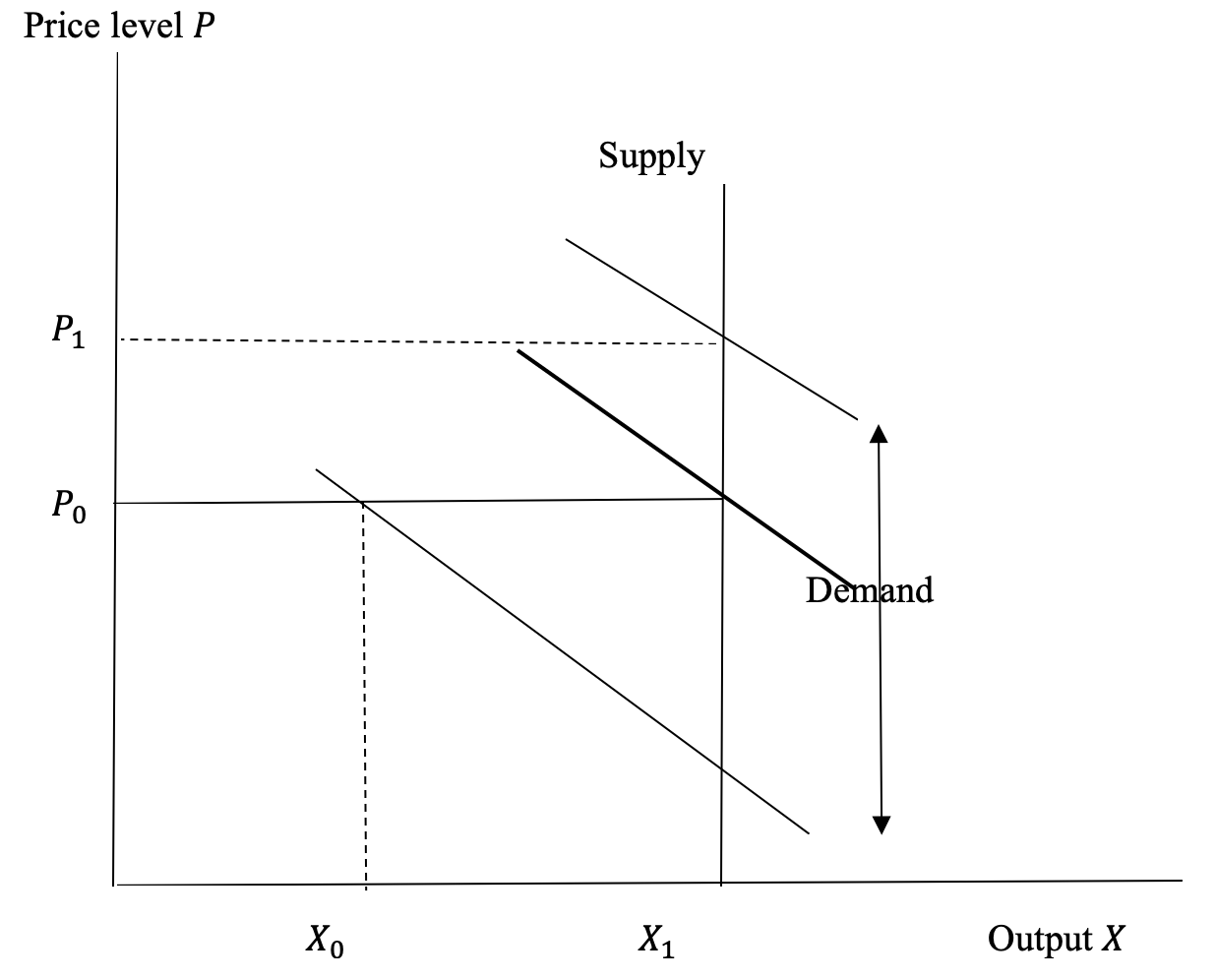
Figure 3: Price level determination
Traditional “inflation” theory
Wicksell had already pointed out that inflation is a “cumulative process” involving feedback between price and wage inflation rates. Even after their long decline, labor payments still make up over half of US production costs and have to enter inflation accounting. Figure 3 is a common non-Wicksellian illustration of how the price level (not the growth rate of prices, or inflation) might be determined. The diagram’s key assumption is that the nominal cost of production (a mark-up on the money wage) is constant when output is below the “full capacity” level X1. A relatively low level of demand will peg output at X0 and the price level at
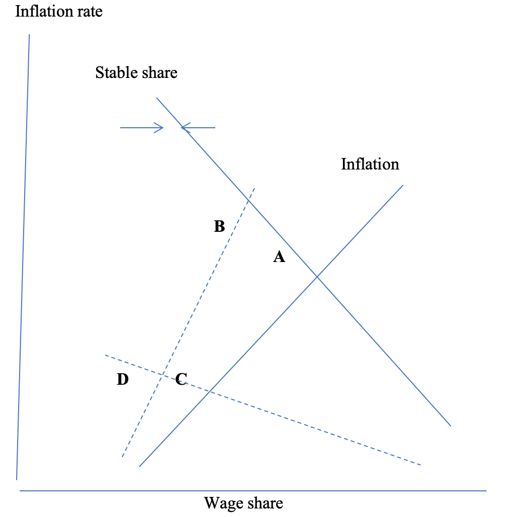
Figure 4: Inflation dynamics
In an overall inflationary environment, business can respond immediately to increases in the wage share or output by pushing up the rate of price increase in Phillips curve fashion along the “Inflation” schedule. Money wages on the other hand are not immediately indexed à la Friedman to price inflation so that they will follow with a lag. Labor will push for faster wage inflation when the wage share is low. The “Stable share” schedule with a negative slope will emerge from this bargaining. It will be steeper, the stronger is labor’s market power. The small arrows show that if the labor share is low (or high) then it will tend to rise (or fall) until it hits the stability curve.
Suppose that there is an initial inflation equilibrium at point A. Using fiscal or monetary policy to stimulate aggregate demand would shift the inflation locus upward (dashed line) with more rapid inflation and a somewhat lower wage share in macro equilibrium at B along the Stable share schedule. Outcomes would be similar if prices rise in “flex-price” markets for specific goods and services. Depending on wage responses, ongoing inflation could result.[2]
Alternatively, under wage repression, the ability of workers to attain a high wage share could be weak, as illustrated by the dashed stability locus with a shallow slope. In response to expansionary policy beginning at C, there would be a modest increase in inflation and a substantially lower wage share ending up at D. Wage repression would stave off inflation under any fiscal or monetary expansion or upward movements of flex-prices.
The way that expansionary policy could pay off in terms of inequality and (possibly) faster inflation would be through an upward shift in the Stable share schedule if the labor market tightens. Even though measured unemployment plummeted over the past decade (especially with Covid), underemployment remains as Fontanari et.al. (2021) observe. There has been a big employment shift (14% of the labor force between 1990 and the mid-2000) toward producing sectors with low wages and productivity and slow productivity growth (Taylor with Ömer, 2020). Aggressive demand stimulus could reverse this trend. Obviously, there are complicating factors, but a useful summary of the model is that the incoming Biden administration faces a trilemma among income distribution, inflation, and the returns to and prices of assets.
Econometrics
Before getting to Biden’s potential problems with inflation it makes sense to sketch econometric results for a properly specified structuralist Phillips curve and take up interactions between the interest rate and asset prices.
To sharpen intuition about inflation dynamics, look back at Figure 2. After 1990, subject to cyclical fluctuations, the labor share of gross income fell by four or five percentage points (pp). The GDP deflator fell by about two pp and wage inflation by more. There appears to be a robust linkage between a falling labor income share and slower inflation. To pursue this connection further, Taylor and Barbosa-Filho (2021) work with a model of consumer price inflation, import price inflation, the unemployment rate, and the labor share of net domestic income. Standard tests show that all four variables are stationary, so that “vector error correction” estimation of a “cointegrating” equation among the variables is appropriate.
It shows that between 1991 and 2019, a one pp increase in import prices pushed up US consumer prices approximately 0.207 pp. The coefficient for the rate of unemployment has the “wrong sign”, i. e., an increase in the rate raised inflation in 1991-2019, but its value is low and not statistically significant, even at 10%. In contrast, the coefficient for the labor share is statistically significant at 1% and mathematically relevant. Assuming everything else constant, a one pp increase in the labor share tended to raise consumer inflation by approximately 0.188 pp in 1991-2019.[3] The USA had no Phillips curve as usually specified. It does seem to have followed a structuralist curve, in which inflation responded to the labor share which in turn reacted cyclically to the rate of unemployment.
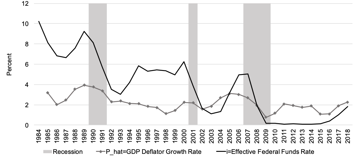
Figure 5: Inflation vs. short-term Fed funds interest rate. Look at how closely the rate tracks the deflator.
Figure 5 shows how the interest rate trails the GDP deflator. Three aspects are relevant to policy. One is Fed interest rate tracking, already discussed. Another is that arbitrage relationships within the bond market force interest rates (the term structure) to follow inflation more or less closely.
The third dates back to the days of Alan Greenspan as Governor of the Fed (1987-2006). After the dot-com bubbles burst in 2000 he instituted a policy of holding rates down whenever asset prices, especially on the stock market, wobbled. In a process that economists call capitalization, a lower interest rate will tend to increase the net present value of an asset’s returns over time, thus raising its market valuation (the financial press has recently been full of discussion of this phenomenon). Wall Street and rich households reap the gains. The mechanism will play a crucial role in policy formation
Complications with policy
Wealth changes are certainly one factor complicating policy. Low interest rates have supported huge capital value increases which mostly accrued to the top ten percent of households in the income size distribution.
Marketing for the Fed policy of holding interest rates down is that the rise in spending power due to asset price increases is supposed to stimulate consumption demand. Between 2016 and 2020 stock market and household equity rose by about $2.5 trillion per year in a $20 trillion economy. A typical estimate of consumption from higher wealth is four percent, implying a trivial consumption boost of around $100 billion per year.
Another channel for transfers to the affluent takes the form of stock buybacks by S&P 500 firms. Before Covid, they shot up to close to a trillion dollars per year. After 2008, non-financial corporate debt rose by $2.8 trillion while S&P firms’ buybacks totaled $5.4 trillion. Evidently, business tapped profits, debt, and recently the proceeds from the Trump tax cut to buy up their own equity. This portfolio shift toward households probably added a few tens of billions to the consumption boost.
Now contrast the position of households in the bottom deciles of the size distribution. They have low positive or negative saving rates – demand in the USA is “low-income led” (Taylor with Ömer, 2020). Suppose poor households were transferred $2.5 trillion. Because they are “taxed” at over thirty percent in terms of reduced benefits when they get extra money, they might spend well over an extra trillion on consumption – an order of magnitude higher than affluent households. Using capital gains and tax-cut financed share buybacks to support aggregate demand is both inefficient and unethical.
Fiscal debt is another fear in the background. There is a potential danger because greater labor militancy could drive up the inflation and real interest rates and cause debt growth to increase, with potentially difficult consequences for the Treasury. Capital flight would be possible but unlikely because the almighty dollar remains the dominant store of international wealth.
More immediately, given the increasing impact of imports on unit costs illustrated in Figure 1, the US exchange rate (dollars per unit of foreign currency) plays a role.[4] A devaluation or increase in the rate will drive up supply cost directly, but also reduce wage cost per unit output. In addition, dollar devaluation tends to drive up commodity prices, giving another inflationary push. The push could be boosted by a commodity price “supercycle” which may be emerging (the last one was roughly between 2000 and 2010 – see the rising import costs in Figure 1).
To take just one example of the policy impact, in 1994 there was maneuvering within the Treasury for modest devaluation. To protect its transaction fees, Wall Street immediately went to incoming Secretary Robert Rubin who pronounced that “A strong dollar is in our national interest,” and instituted an anti-inflationary Strong Dollar Policy which persists today.
The Biden Trilemma
What policy options does the Biden administration have? For several years, money wage growth would have to exceed productivity growth by one pp annually for the Fed to attain a target of three percent price inflation. Translating that goal into policy underlines the difficulties of a trilemma that the team faces. There are contradictions among three competing objectives, already subject to the difficulties just mentioned:
First, money wage growth must exceed the sum of growth rates of prices and productivity if the huge increase in inequality in the size distribution of income since 1970 is ever to be reversed. Low incomes depend heavily on wages and fiscal transfers, and political possibilities for increases in the latter are likely to be limited.
Consequently, the inflation rate would increase as firms pass higher costs into higher prices. The Fed’s two percent target could be breached, at which point the authorities could well move toward demand contraction.
Finally, for the reasons discussed in connection with Figure 5, faster inflation would drive up interest rates, forcing asset prices down, driving up costs of servicing private and fiscal debt, and cutting into financial fees. Strong reactions (at the very least) could be expected from Wall Street and affluent households. The Fed’s floor under interest rates when asset prices wobble could well be a flashpoint. It has been in place now for 35 years and is almost Holy Writ for Wall Street.
Future prospects?
The Biden administration’s economic priorities seem clear. With the potential inflation trilemma, achieving them will be a tremendously difficult task, even ignoring the numerous other complications.
The labor market shows signs of tightening as of June 2021 (Furman and Powell, 2021). Even standard estimates suggest a big gap between potential and actual output, while both job openings and quit rates are high. Even more significant is that average wage rates were growing at almost ten percent per year. If that trend persists (it may be sensitive to both a low base level for the estimation and compositional effects across sectors) there could be substantial cost-push inflation pressure.
Import complications have already been noted. On a trade-weighted basis, the dollar has depreciated by about ten percent since hitting a peak in March 2020. One impact could be an increase in commodity prices, beyond any potential supercycle.[5] For foreign asset holders, a weak dollar means that American liabilities are cheap but the expected return from dollar appreciation to purchasing them is anybody’s guess. That is why forecasting exchange rate movements is very difficult. The bottom line is that import prices could rise, adding to inflationary pressure and interest rate increases.
In sum, from the side of costs, a Wicksellian cumulative inflation process is a possibility. Whether it can establish itself is the key question. There are certainly indicators that it will not, e.g., the collapse of the Amazon union drive in April 2021, failures on minimum wage legislation, and for that matter the absence of aggressive strike behavior. There would be a stronger case for worry about inflation if those events had gone the other way. Time will tell.
Biden’s bet
Biden’s policy line appears to be that productivity will grow fast, thanks to rapid demand expansion and the Verdoorn effect mentioned above. Money wages could then increase more rapidly than the price level without provoking inflation. The real wage could rise, although implicitly the distributional goal of an increasing labor share would have to be abandoned because that requires wages to grow faster than the price level plus productivity. Biden’s bet is that his expansion will be inflationary, not too much, and not for too long. How much the labor share can be further reduced is the skeleton key to the trilemma.
Support from INET and comments from Thomas Ferguson are gratefully acknowledged
References
Barbosa-Filho, Nelson H. (2008) “Verdoorn’s Law,” Encyclopedia.com https://www.encyclopedia.com/social-sciences/applied-and-social-sciences-magazines/verdoorns-law
Barbosa-Filho, Nelson H., and Lance Taylor (2006) “Distributive and Demand Cycles in the U.S. Economy – A Structuralist Goodwin Model, Metroeconomica, 57: 389-411
Cardoso, Eliana (1981) “Food Supply and Inflation,” Journal of Development Economics, 8: 269-284
Fontanari, Claudia, Antonella Palumbo, and Chiara Salvatoti (2021) “Slack in the Economy, Not Inflation, Should be the Bigger Worry,” Institute for New Economic Thinking, https://www.ineteconomics.org/perspectives/blog/slack-in-the-economy-not-inflation-should-be-bigger-worry
Friedman, Milton (1968) “The Role of Monetary Policy,” American Economic Review, 58: 1-17.
Furman, Jason, and Wilson Powell III (2021) “US Labor Market Heated Up in May as Jobs Grew and Wages Soared,” https://www.piie.com/blogs/realtime-economic-issues-watch/us-labor-market-heated-may-jobs-grew-and-wages-soared
Keynes, John Maynard (1936) The General Theory of Employment, Interest, and Money, London: Macmillan.
Hicks, John R. (1932) The Theory of Wages, London; Macmillan.
Okun, Arthur (1962) “Potential GNP: Its Measurement and Significance,” Proceedings of the American Statistical Association, Business and Economic Statistics Section, ASA Washington, 98-104.
Phillips, William (1958) “The Relationship Between Unemployment and the Rate of Change of Money Wage Rates in the United Kingdom 1861-1957,” Economica, 25: 283-299.
Samuelson, Paul A., and Robert M. Solow (1960) “Analytical Aspects of Anti-Inflation Policy,” American Economic Review (Papers and Proceedings), 50(2): 177-194.
Sunkel, Oswaldo (1960) “Inflation in Chile: An Unorthodox Approach,” International Economic Papers, No. 10, 107-131.
Taylor, Lance and Nelson H. Barbosa-Filho (2021) “Inflation? It’s Import Prices and the Labor Share,” Institute for New Economic Thinking Working Paper No. 145, https://www.ineteconomics.org/research/research-papers/inflation-its-import-prices-and-the-labor-share
Taylor, Lance, with Özlem Ömer (2020) Macroeconomic Inequality from Reagan to Trump: Market Power, Wage Repression, Price Inflation, and Industrial Decline, New York: Cambridge University Press.
Endnotes
[1] His example was the famous “beauty contest” in which participants were asked to pick the newspaper photo of a young woman which all players would consider to be the prettiest among a group.
[2] This idea dates back to Latin American food price inflation theory (Sunkel, 1960). Cardoso (1981) provides an elegant model. Hicks (1932) talked about “fix-price” and “flex-price” markets. As of mid-2021, flex-price behavior became more common in specific markets across the American economy.
[3] The effect is roughly half as strong as one would infer from eyeballing Figure 2.
[4] Although it is confusing, this definition of the exchange rate is standard in open economy macroeconomics.
[5] Commodity prices are mostly quoted in dollars. US devaluation means that international producers’ incomes fall so they tend to push up prices.